 Calculate Critical Z Value

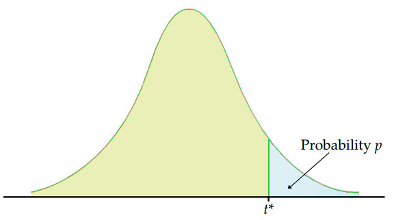
Enter a probability value between zero and one to calculate critical value. Critical values determine what probability a particular variable will have when a sampling distribution is normal or close to normal.
Formula:
Probability (p): p = 1 - α/2.
Critical Value: Definition and Significance in the Real World
- Guide Authored by Corin B. Arenas, published on October 4, 2019
Ever wondered if election surveys are accurate? How about statistics on housing, health care, and testing scores?
In this section, we’ll discuss how sample data is tested for accuracy. Read on to learn more about critical value, how it’s used in statistics, and its significance in social science research.
What is a Critical Value?

In testing statistics, a critical value is a factor that determines the margin of error in a distribution graph.
According to Statistics How To, a site headed by math educator Stephanie Glen, if the absolute value of a test statistic is greater than the critical value, then there is statistical significance that rejects an accepted hypothesis.
Critical values divide a distribution graph into sections which indicate ‘rejection regions.’ Basically, if a test value falls within a rejection region, it means an accepted hypothesis (referred to as a null hypothesis) must be rejected. And if the test value falls within the accepted range, the null hypothesis cannot be rejected.
Testing sample data involves validating research and surveys like voting habits, SAT scores, body fat percentage, blood pressure, and all sorts of population data.
Hypothesis Testing and the Distribution Curve

Hypothesis tests check if your data was taken from a sample population that adheres to a hypothesized probability distribution. It is characterized by a null hypothesis and an alternative hypothesis.
In hypothesis testing, a critical value is a point on a distribution graph that is analyzed alongside a test statistic to confirm if a null hypothesis—a commonly accepted fact in a study which researchers aim to disprove—should be rejected.
The value of a null hypothesis implies that no statistical significance exists in a set of given observations. It is assumed to be true unless statistical evidence from an alternative hypothesis invalidates it.
How does this relate with distribution graphs? A normal distribution curve, which is a bell-shaped curve, is a theoretical representation of how often an experiment will yield a particular result.
Elements of Normal Distribution:
- Has a mean, median, or mode. A mean is the average of numbers in a group, a median is the middle number in a list of numbers, and a mode is a number that appears most often in a set of numbers.
- 50% of the values are less than the mean
- 50% of the values are greater than the mean
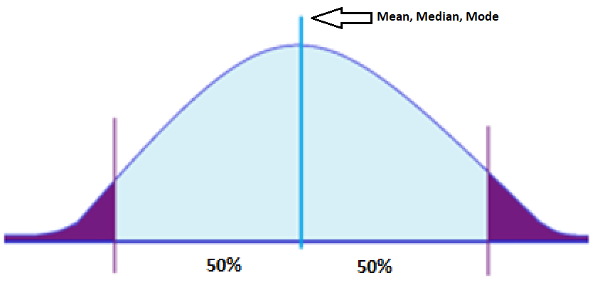
Majority of the data points in normal distribution are relatively similar. A perfectly normal distribution is characterized by its symmetry, meaning half of the data observations fall on either side of the middle of the graph. This implies that they occur within a range of values with fewer outliers on the high and low points of the graph.
Given these implications, critical values do not fall within the range of common data points. Which is why when a test statistic exceeds the critical value, a null hypothesis is forfeited.
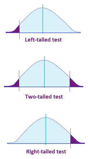
Take note: Critical values may look for a two-tailed test or one-tailed test (right-tailed or left-tailed). Depending on the data, statisticians determine which test to perform first.
Finding the Critical Value

The standard equation for the probability of a critical value is:
p = 1 – α/2
Where p is the probability and alpha (α) represents the significance or confidence level. This establishes how far off a researcher will draw the line from the null hypothesis.
The alpha functions as the alternative hypothesis. It signifies the probability of rejecting the null hypothesis when it is true. For instance, if a researcher wants to establish a significance level of 0.05, it means there is a 5% chance of finding that a difference exists.
When the sampling distribution of a data set is normal or close to normal, the critical value can be determined as a z score or t score.
Z Score or T Score: Which Should You Use?
Typically, when a sample size is big (more than 40) using z or t statistics is fine. However, while both methods compute similar results, most beginner’s textbooks on statistics use the z score.
When a sample size is small and the standard deviation of a population is unknown, the t score is used. The t score is a probability distribution that allows statisticians to perform analyses on specific data sets using normal distribution. But take note: Small samples from populations that are not approximately normal should not use the t score.
What’s a standard deviation? This measures how numbers are spread out in a set of values, showing the amount of variation. Low standard deviation means the numbers are close to the mean set, while a high standard deviation signifies numbers are dispersed at a wider range.
Calculating Z Score
The critical value of a z score can be used to determine the margin of error, as shown in the equations below:
- Margin of error = Critical value x Standard deviation of the statistic
- Margin of error = Critical value x Standard error of the statistic
The z score, also known as the standard normal probability score, signifies how many standard deviations a statistical element is from the mean. A z score table is used in hypothesis testing to check proportions and the difference between two means. Z tables indicate what percentage of the statistics is under the curve at any given point.
| cumulative prob | t .50 | t .75 | t .80 | t .85 | t .90 | t .95 | t.975 | t .98 | t .99 | t .995 | t . 9975 | t .999 | t .9995 |
|---|---|---|---|---|---|---|---|---|---|---|---|---|---|
| α 1-tail | .5 | .25 | .20 | .15 | .10 | .05 | .025 | .02 | .01 | .005 | .0025 | .001 | .0005 |
| α 2-tail | 1 | .50 | .40 | .30 | .20 | .10 | .050 | .04 | .02 | .010 | .0050 | .002 | .0010 |
| df | |||||||||||||
| z | 0.00 | 0.674 | 0.841 | 1.036 | 1.282 | 1.645 | 1.960 | 2.054 | 2.326 | 2.576 | 2.807 | 3.091 | 3.291 |
| 1 | 0.00 | 1.000 | 1.376 | 1.963 | 3.078 | 6.314 | 12.71 | 15.89 | 31.82 | 63.66 | 127.3 | 318.3 | 636.6 |
| 2 | 0.00 | 0.816 | 1.061 | 1.386 | 1.886 | 2.920 | 4.303 | 4.849 | 6.965 | 9.925 | 14.09 | 22.33 | 31.60 |
| 3 | 0.00 | 0.765 | 0.978 | 1.250 | 1.638 | 2.353 | 3.182 | 3.482 | 4.541 | 5.841 | 7.453 | 10.21 | 12.92 |
| 4 | 0.00 | 0.741 | 0.941 | 1.190 | 1.533 | 2.132 | 2.776 | 2.999 | 3.747 | 4.604 | 5.598 | 7.173 | 8.610 |
| 5 | 0.00 | 0.727 | 0.920 | 1.156 | 1.476 | 2.015 | 2.571 | 2.757 | 3.365 | 4.032 | 4.773 | 5.893 | 6.869 |
| 6 | 0.00 | 0.718 | 0.906 | 1.134 | 1.440 | 1.943 | 2.447 | 2.612 | 3.143 | 3.707 | 4.317 | 5.208 | 5.959 |
| 7 | 0.00 | 0.711 | 0.896 | 1.119 | 1.415 | 1.895 | 2.365 | 2.517 | 2.998 | 3.499 | 4.029 | 4.785 | 5.408 |
| 8 | 0.00 | 0.706 | 0.889 | 1.108 | 1.397 | 1.860 | 2.306 | 2.449 | 2.896 | 3.355 | 3.833 | 4.501 | 5.041 |
| 9 | 0.00 | 0.703 | 0.883 | 1.100 | 1.383 | 1.833 | 2.262 | 2.398 | 2.821 | 3.250 | 3.690 | 4.297 | 4.781 |
| 10 | 0.00 | 0.700 | 0.879 | 1.093 | 1.372 | 1.812 | 2.228 | 2.359 | 2.764 | 3.169 | 3.581 | 4.144 | 4.587 |
| 11 | 0.00 | 0.697 | 0.876 | 1.088 | 1.363 | 1.796 | 2.201 | 2.328 | 2.718 | 3.106 | 3.497 | 4.025 | 4.437 |
| 12 | 0.00 | 0.695 | 0.873 | 1.083 | 1.356 | 1.782 | 2.179 | 2.303 | 2.681 | 3.055 | 3.428 | 3.930 | 4.318 |
| 13 | 0.00 | 0.694 | 0.870 | 1.079 | 1.350 | 1.771 | 2.160 | 2.282 | 2.650 | 3.012 | 3.372 | 3.852 | 4.221 |
| 14 | 0.00 | 0.692 | 0.868 | 1.076 | 1.345 | 1.761 | 2.145 | 2.264 | 2.624 | 2.977 | 3.326 | 3.787 | 4.140 |
| 15 | 0.00 | 0.691 | 0.866 | 1.074 | 1.341 | 1.753 | 2.131 | 2.249 | 2.602 | 2.947 | 3.286 | 3.733 | 4.073 |
| 16 | 0.00 | 0.690 | 0.865 | 1.071 | 1.337 | 1.746 | 2.120 | 2.235 | 2.583 | 2.921 | 3.252 | 3.686 | 4.015 |
| 17 | 0.00 | 0.689 | 0.863 | 1.069 | 1.333 | 1.740 | 2.110 | 2.224 | 2.567 | 2.898 | 3.222 | 3.646 | 3.965 |
| 18 | 0.00 | 0.688 | 0.862 | 1.067 | 1.330 | 1.734 | 2.101 | 2.214 | 2.552 | 2.878 | 3.197 | 3.611 | 3.922 |
| 19 | 0.00 | 0.688 | 0.861 | 1.066 | 1.328 | 1.729 | 2.093 | 2.205 | 2.539 | 2.861 | 3.174 | 3.579 | 3.883 |
| 20 | 0.00 | 0.687 | 0.860 | 1.064 | 1.325 | 1.725 | 2.086 | 2.197 | 2.528 | 2.845 | 3.153 | 3.552 | 3.850 |
| 21 | 0.00 | 0.686 | 0.859 | 1.063 | 1.323 | 1.721 | 2.080 | 2.189 | 2.518 | 2.831 | 3.135 | 3.527 | 3.819 |
| 22 | 0.00 | 0.686 | 0.858 | 1.061 | 1.321 | 1.717 | 2.074 | 2.183 | 2.508 | 2.819 | 3.119 | 3.505 | 3.792 |
| 23 | 0.00 | 0.685 | 0.858 | 1.060 | 1.319 | 1.714 | 2.069 | 2.177 | 2.500 | 2.807 | 3.104 | 3.485 | 3.768 |
| 24 | 0.00 | 0.685 | 0.857 | 1.059 | 1.318 | 1.711 | 2.064 | 2.172 | 2.492 | 2.797 | 3.091 | 3.467 | 3.745 |
| 25 | 0.00 | 0.684 | 0.856 | 1.058 | 1.316 | 1.708 | 2.060 | 2.167 | 2.485 | 2.787 | 3.078 | 3.450 | 3.725 |
| 26 | 0.00 | 0.684 | 0.856 | 1.058 | 1.315 | 1.706 | 2.056 | 2.162 | 2.479 | 2.779 | 3.067 | 3.435 | 3.707 |
| 27 | 0.00 | 0.684 | 0.855 | 1.057 | 1.314 | 1.703 | 2.052 | 2.158 | 2.473 | 2.771 | 3.057 | 3.421 | 3.690 |
| 28 | 0.00 | 0.683 | 0.855 | 1.056 | 1.313 | 1.701 | 2.048 | 2.154 | 2.467 | 2.763 | 3.047 | 3.408 | 3.674 |
| 29 | 0.00 | 0.683 | 0.854 | 1.055 | 1.311 | 1.699 | 2.045 | 2.150 | 2.462 | 2.756 | 3.038 | 3.396 | 3.659 |
| 30 | 0.00 | 0.683 | 0.854 | 1.055 | 1.310 | 1.697 | 2.042 | 2.147 | 2.457 | 2.750 | 3.030 | 3.385 | 3.646 |
| 40 | 0.00 | 0.681 | 0.851 | 1.050 | 1.303 | 1.684 | 2.021 | 2.123 | 2.423 | 2.704 | 2.971 | 3.307 | 3.551 |
| 50 | 0.00 | 0.679 | 0.849 | 1.047 | 1.299 | 1.676 | 2.009 | 2.109 | 2.403 | 2.678 | 2.937 | 3.261 | 3.496 |
| 60 | 0.00 | 0.679 | 0.848 | 1.045 | 1.296 | 1.671 | 2.000 | 2.099 | 2.390 | 2.660 | 2.915 | 3.232 | 3.460 |
| 80 | 0.00 | 0.678 | 0.846 | 1.043 | 1.292 | 1.664 | 1.990 | 2.088 | 2.374 | 2.639 | 2.887 | 3.195 | 3.416 |
| 100 | 0.00 | 0.677 | 0.845 | 1.042 | 1.290 | 1.660 | 1.984 | 2.081 | 2.364 | 2.626 | 2.871 | 3.174 | 3.390 |
| 1000 | 0.00 | 0.675 | 0.842 | 1.037 | 1.282 | 1.646 | 1.962 | 2.056 | 2.330 | 2.581 | 2.813 | 3.098 | 3.300 |
| 0% | 50% | 60% | 70% | 80% | 90% | 95% | 96% | 98% | 99% | 99.5% | 99.8% | 99.9% |
The basic formula for a z score sample is:
z = (X – μ) / σ
Where,
- X is the value of the element
- μ is the population mean
- σ is the standard deviation
Let’s solve an example. For instance, let’s say you have a test score of 85. If the test has a mean (μ) of 45 and a standard deviation (σ) of 23, what’s your z score?
X = 85, μ = 45, σ = 23
z = (85 – 45) / 23
= 40 / 23
z = 1.7391
For this example, your score is 1.7391 standard deviations above the mean.
What do the z scores imply?
- If a score is greater than 0, the statistic sample is greater than the mean
- If the score is less than 0, the statistic sample is less than the mean
- If a score is equal to 1, it means the sample is 1 standard deviation greater than the mean, and so on
- If a score is equal to -1, it means the sample is 1 standard deviation less than the mean, and so on
For elements in a large set:
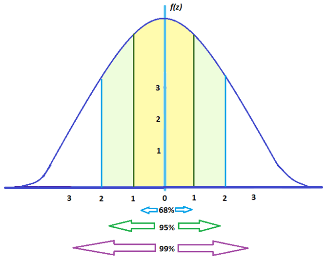
- Around 68% fall between -1 and 1
- Around 95% fall between -2 and 2
- Around 99% fall between -3 and 3
To give you an idea, here’s how spread out statistical elements would look like under a z score graph:
Calculating T Score
On the other hand, here’s the standard formula for the t score:
t = [ x – μ ] / [ s / sqrt( n ) ]
Where,
- x is the sample mean
- μ is the population mean
- s is the sample’s standard deviation
- n is the sample size
Then, we account for the degrees of freedom (df) which is the sample size minus 1. df = n – 1
T distribution, also known as the student’s distribution, is associated with a unique cumulative probability. This signifies the chance of finding a sample mean that’s less than or equal to x, based on a random sample size n. Cumulative probability refers to the likelihood that a random variable would fall within a specific range. To express the t statistic with a cumulative probability of 1 – α, statisticians use tα.
Part of finding the t score is locating the degrees of freedom (df) using the t distribution table as a reference. For demonstration purposes, let’s say you have a small sample of 5 and you want to conduct a right-tailed test. Follow the steps below.
5 df, α = 0.05
- Take your sample size and subtract 1. 5 – 1 = 4. df = 4
- For this example, let’s say the alpha level is 5% (0.05).
- Look for the df in the t distribution table along with its corresponding alpha level. You’ll find the critical value where the column and row intersect.
| df | α = 0.1 | 0.05 | 0.025 | 0.01 | 0.005 |
| ∞ | ta= 1.2816 | 1.6449 | 1.96 | 2.3263 | 2.5758 |
| 1 | 3.078 | 6.314 | 12.706 | 31.821 | 63.656 |
| 2 | 1.886 | 2.920 | 4.303 | 6.965 | 9.925 |
| 3 | 1.638 | 2.353 | 3.182 | 4.541 | 5.841 |
| 4 | 1.533 | 2.132 | 2.776 | 3.747 | 4.604 |
| 5 | 1.476 | 2.015 | 2.571 | 3.365 | 4.032 |
*One-tail t distribution table referenced from How to Statistics.
In this example, 5 df, α = 0.05, the critical value is 2.132.
Here’s another example using the t score formula.
A factory produces CFL light bulbs. The owner says that CFL bulbs from their factory lasts for 160 days. Quality specialists randomly chose 20 bulbs for testing, which lasted for an average of 150 days, with a standard deviation of 40 days. If the CFL bulbs really last for 160 days, what is the probability that 20 random CFL bulbs would have an average life that’s less than 150 days?
t = [ x – μ ] / [ s / sqrt( n ) ]
- x = 150
- μ = 160
- s = 40
- n = 20
t = [ 150 – 160 ] / [ 40 / sqrt( 20 ) ]
= -10 / [40 / 4.472135]
= -10 / 8.94427
t = -1.118034
The degrees of freedom: df = 20 – 1, df = 19
Again, use the variables above to refer to a t distribution table, or use a t score calculator.
For this example, the critical value is 0.1387. Thus, if the life of a CFL light bulb is 160 days, there is a 13.87% probability that the average CFL bulb for 20 randomly chosen bulbs would be less than or equal to 150 days.
If we were to plot the critical value and shade the rejection region in a graph, it would look like this:
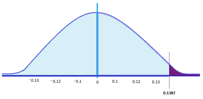
If a test statistic is greater than this critical value, then the null hypothesis, which is ‘CFL light bulbs have a life of 160 days,’ should be rejected. That’s if tests show more than 13.87% of the sample light bulbs (20) have a lifespan of less than or equal 150 days.
Why is Determining Critical Value Important?
Researchers often work with a sample population, which is a small percentage when they gather statistics.
Working with sample populations does not guarantee that it reflects the actual population’s results. To test if the data is representative of the actual population, researchers conduct hypothesis testing which make use of critical values.
What are Real-World Uses for It?

Validating statistical knowledge is important in the study of a wide range of fields. This includes research in social sciences such as economics, psychology, sociology, political science, and anthropology.
For one, it keeps quality management in check. This includes product testing in companies and analyzing test scores in educational institutions.
Moreover, hypothesis testing is crucial for the scientific and medical community because it is imperative for the advancement of theories and ideas.
If you’ve come across research that studies behavior, then the study likely used hypothesis testing and sampling in populations. From the public’s voting behavior, to what type of houses people tend to buy, researchers conduct distribution tests.
Studies such as how male adolescents in certain states are prone to violence, or how children of obese parents are prone to becoming obese, are other examples that use critical values in distribution testing.
In the field of health care, topics like how often diseases like measles, diphtheria, or polio occur in an area is relevant for public safety. Testing would help communities know if there are certain health conditions rising at an alarming rate. This is especially relevant now in the age of anti-vaccine activists.
The Bottom Line
Finding critical values are important for testing statistical data. It’s one of the main factors in hypothesis testing, which can validate or disprove commonly accepted information.
Proper analysis and testing of statistics help guide the public, which corrects misleading or dated information.
Hypothesis testing is useful in a wide range of disciplines, such as medicine, sociology, political science, and quality management in companies.
About the Author
Corin is an ardent researcher and writer of financial topics—studying economic trends, how they affect populations, as well as how to help consumers make wiser financial decisions. Her other feature articles can be read on Inquirer.net and Manileno.com. She holds a Master’s degree in Creative Writing from the University of the Philippines, one of the top academic institutions in the world, and a Bachelor’s in Communication Arts from Miriam College.
How to Excel at Math Cartoon


